Table of Contents >> Show >> Hide
- What Is Expected Opportunity Loss?
- EOL vs. EMV: What Is the Difference?
- How to Calculate Expected Opportunity Loss (EOL): 13 Steps
- Step 1: Define the Decision Problem
- Step 2: List the Decision Alternatives
- Step 3: Identify the States of Nature
- Step 4: Assign Probabilities to the States of Nature
- Step 5: Build the Payoff Table
- Step 6: Find the Best Payoff for Each State of Nature
- Step 7: Calculate Opportunity Loss for Each Cell
- Step 8: Create the Opportunity Loss Table
- Step 9: Multiply Each Opportunity Loss by Its Probability
- Step 10: Add the Weighted Losses for Each Alternative
- Step 11: Compare the EOL Result with EMV
- Step 12: Connect EOL to EVPI
- Step 13: Interpret the Result Before Making the Final Decision
- Common Mistakes When Calculating EOL
- When Should You Use Expected Opportunity Loss?
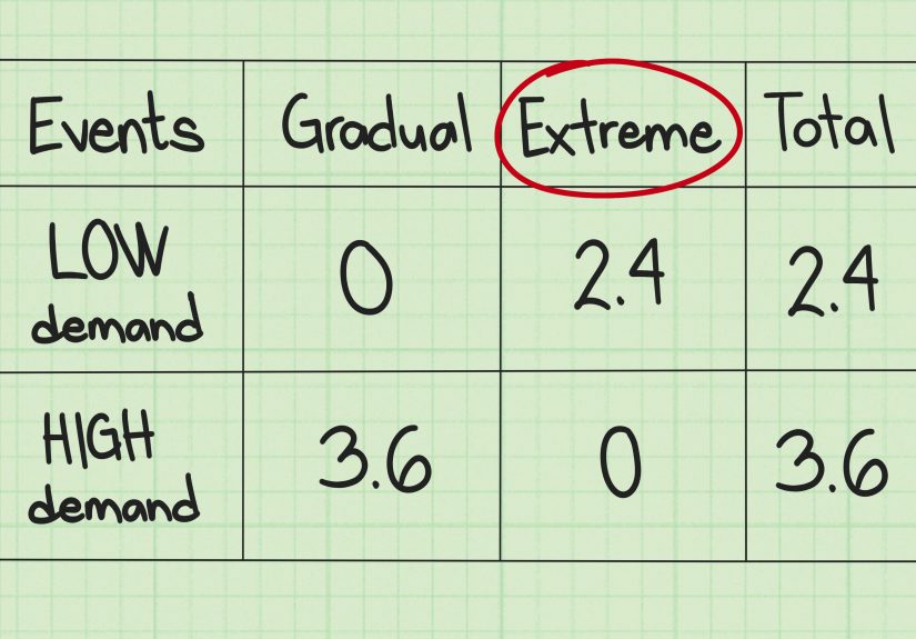
- Practical Example: Inventory Planning
- Experience-Based Tips for Calculating EOL Better
- Conclusion
Expected Opportunity Loss, or EOL, sounds like something your spreadsheet mutters when you make a questionable business decision at 11:47 p.m. Fortunately, it is much friendlier than it sounds. EOL is a decision-making tool that helps you compare choices when the future is uncertain. Instead of asking, “How much could I make?” it asks, “How much would I regret losing if another choice turned out to be better?”
That may sound dramatic, but it is incredibly practical. Businesses use Expected Opportunity Loss in decision analysis, finance, operations management, inventory planning, project evaluation, and risk assessment. Students meet it in statistics, business math, economics, and quantitative analysis. Managers use it when deciding whether to launch a product, expand a facility, stock inventory, buy information, or choose between competing investments.
The beauty of EOL is that it turns regret into math. Instead of relying on gut feelings, crossed fingers, or the legendary “my cousin said this is a sure thing” method, you build a payoff table, calculate what you would miss out on under each possible future, multiply those losses by probability, and choose the option with the lowest expected loss. Neat, logical, and much less messy than arguing in a conference room with stale donuts.
What Is Expected Opportunity Loss?
Expected Opportunity Loss (EOL) is the weighted average of the opportunity losses, or regrets, associated with a decision alternative. In plain English, it estimates how much value you expect to lose by choosing one option instead of the best option for each possible future outcome.
An opportunity loss happens when you choose an alternative and later discover that another alternative would have produced a better payoff. The difference between the best possible payoff and the payoff from your chosen decision is the opportunity loss.
The basic formula is:
EOL = Σ (Opportunity Loss for each state of nature × Probability of that state)
The decision rule is simple:
Choose the alternative with the lowest Expected Opportunity Loss.
EOL is also called expected regret because it measures the expected cost of not making the best decision after the future becomes known. Of course, real life rarely sends you a polite memo titled “Correct Answer Attached,” so EOL helps you make the best decision before the future arrives wearing sunglasses and refusing to explain itself.
EOL vs. EMV: What Is the Difference?
Expected Monetary Value (EMV) focuses on the expected payoff of each decision. You multiply each payoff by its probability, add the results, and choose the alternative with the highest expected value.
Expected Opportunity Loss looks at the same problem from the opposite angle. Instead of calculating expected gain, it calculates expected regret. In many standard profit-based decision problems, choosing the minimum EOL alternative leads to the same decision as choosing the maximum EMV alternative. The difference is perspective: EMV says, “What do I expect to earn?” EOL says, “What do I expect to miss?”
Both methods are useful. EMV is direct and profit-focused. EOL is especially helpful when you want to understand the cost of uncertainty or explain why additional research, forecasting, or market information may be worth buying.
How to Calculate Expected Opportunity Loss (EOL): 13 Steps
Step 1: Define the Decision Problem
Start by writing down the decision you need to make. Keep it specific. “Should we expand?” is better than “What should we do with the business?” A clear decision problem makes the rest of the EOL calculation much easier.
Example: A company must choose one of three strategies: expand operations, renovate the current facility, or do nothing.
Step 2: List the Decision Alternatives
Your decision alternatives are the actions you can choose. Put them in rows. These should be mutually exclusive options when possible, meaning you will choose one main path.
- Expand
- Renovate
- Do nothing
Do not overload the table with vague choices such as “try harder” or “be innovative.” Those may sound great in a meeting, but they are not decision alternatives unless you can attach measurable outcomes to them.
Step 3: Identify the States of Nature
States of nature are possible future conditions you cannot control. They might include strong demand, weak demand, good economic conditions, bad economic conditions, high interest rates, low interest rates, supplier delays, or competitor actions.
For our example, assume two states of nature:
- Good economic conditions
- Bad economic conditions
The key is that one of these futures will happen, but you do not know which one when making the decision.
Step 4: Assign Probabilities to the States of Nature
EOL is used for decision-making under risk, meaning probabilities are known or can be estimated. Probabilities must add up to 1.00, or 100%.
Example:
- Good economic conditions: 0.60
- Bad economic conditions: 0.40
These probabilities may come from historical data, market research, expert judgment, forecasting models, or a combination of evidence. If the probabilities are wildly guessed, the EOL calculation will still produce a number, but that number may be wearing a fake mustache.
Step 5: Build the Payoff Table
A payoff table shows the payoff for each decision alternative under each state of nature. Payoffs may be profits, costs, savings, revenues, utility scores, or any other measurable outcome. For profit problems, higher numbers are better.
| Decision Alternative | Good Economy | Bad Economy |
|---|---|---|
| Expand | $150,000 | -$10,000 |
| Renovate | $90,000 | $10,000 |
| Do nothing | $70,000 | $40,000 |
This table tells us that expansion performs best when the economy is good, but it performs poorly when the economy is bad. Doing nothing is less exciting, but it holds up better in a downturn. In other words, expansion is the sports car, and doing nothing is the reliable umbrella.
Step 6: Find the Best Payoff for Each State of Nature
For each column, identify the highest payoff. This is the payoff you would choose if you knew that state of nature would occur.
In a good economy, the best payoff is $150,000 from expanding. In a bad economy, the best payoff is $40,000 from doing nothing.
| State of Nature | Best Payoff | Best Alternative |
|---|---|---|
| Good Economy | $150,000 | Expand |
| Bad Economy | $40,000 | Do nothing |
Step 7: Calculate Opportunity Loss for Each Cell
Now create the opportunity loss table. For each state of nature, subtract each payoff from the best payoff in that column.
Opportunity Loss = Best payoff for that state − Payoff for the selected alternative
For the good economy column:
- Expand: $150,000 − $150,000 = $0
- Renovate: $150,000 − $90,000 = $60,000
- Do nothing: $150,000 − $70,000 = $80,000
For the bad economy column:
- Expand: $40,000 − (-$10,000) = $50,000
- Renovate: $40,000 − $10,000 = $30,000
- Do nothing: $40,000 − $40,000 = $0
Step 8: Create the Opportunity Loss Table
The opportunity loss table shows regret values instead of payoffs.
| Decision Alternative | Good Economy Regret | Bad Economy Regret |
|---|---|---|
| Expand | $0 | $50,000 |
| Renovate | $60,000 | $30,000 |
| Do nothing | $80,000 | $0 |
A zero means there is no regret in that state because the decision is the best choice for that future. Larger numbers mean larger missed opportunities.
Step 9: Multiply Each Opportunity Loss by Its Probability
Now weight each regret value by the probability of the related state of nature.
Probabilities:
- Good economy: 0.60
- Bad economy: 0.40
Calculations:
- Expand: ($0 × 0.60) + ($50,000 × 0.40)
- Renovate: ($60,000 × 0.60) + ($30,000 × 0.40)
- Do nothing: ($80,000 × 0.60) + ($0 × 0.40)
Step 10: Add the Weighted Losses for Each Alternative
Add the weighted opportunity losses across each row. This gives the Expected Opportunity Loss for each decision alternative.
| Decision Alternative | EOL Calculation | Expected Opportunity Loss |
|---|---|---|
| Expand | ($0 × 0.60) + ($50,000 × 0.40) | $20,000 |
| Renovate | ($60,000 × 0.60) + ($30,000 × 0.40) | $48,000 |
| Do nothing | ($80,000 × 0.60) + ($0 × 0.40) | $48,000 |
The lowest EOL is $20,000, so the EOL method recommends expanding.
Step 11: Compare the EOL Result with EMV
It is smart to compare EOL with Expected Monetary Value. For the same example:
- Expand EMV = ($150,000 × 0.60) + (-$10,000 × 0.40) = $86,000
- Renovate EMV = ($90,000 × 0.60) + ($10,000 × 0.40) = $58,000
- Do nothing EMV = ($70,000 × 0.60) + ($40,000 × 0.40) = $58,000
The highest EMV is $86,000, which also recommends expanding. EMV and EOL reach the same decision here, but EOL gives extra insight by showing the expected cost of not knowing the future perfectly.
Step 12: Connect EOL to EVPI
Expected Value of Perfect Information (EVPI) is the maximum amount you should be willing to pay for perfect information about which state of nature will occur. In many standard EOL problems, the minimum EOL equals EVPI.
Using the example, the best decision with perfect information would be:
- If the economy is good, expand and earn $150,000.
- If the economy is bad, do nothing and earn $40,000.
Expected value with perfect information:
($150,000 × 0.60) + ($40,000 × 0.40) = $106,000
Best EMV without perfect information:
$86,000
EVPI:
$106,000 − $86,000 = $20,000
The minimum EOL is also $20,000. That means perfect information would be worth up to $20,000 in this decision problem. If a consultant, analyst, or forecasting service charges $50,000 for “perfect” information, politely smile, protect your wallet, and walk away.
Step 13: Interpret the Result Before Making the Final Decision
EOL is powerful, but it is not magic. Before making the final call, ask practical questions:
- Are the probabilities realistic?
- Are the payoff estimates reliable?
- Are there non-financial factors, such as safety, reputation, ethics, or customer trust?
- Is the decision repeated often, or is it a one-time high-stakes choice?
- Would better information change the recommendation?
The lowest EOL gives you the mathematically preferred choice under the assumptions in your model. If the assumptions are weak, update them. A decision model is only as good as the numbers you feed it. Spreadsheets are loyal, but they are not psychic.
Common Mistakes When Calculating EOL
Using Costs Like Profits
If your table shows profits, the best payoff is the highest value in each column. If your table shows costs, the best outcome is the lowest cost. For cost-based tables, opportunity loss is usually calculated by subtracting the lowest cost from each cost value. Mixing up profit logic and cost logic is one of the fastest ways to make your EOL table do interpretive dance.
Forgetting That Probabilities Must Add to 1
If your probabilities add to 0.87 or 1.24, pause immediately. Adjust the probabilities before calculating EOL. Otherwise, your expected loss is distorted.
Choosing the Highest EOL
EOL is a loss measure. Lower is better. Choose the alternative with the minimum EOL, not the maximum. This is not a high-score arcade game.
Confusing Opportunity Loss with Actual Loss
An opportunity loss is not always a cash loss. You might still make money and have opportunity loss if another decision would have made more money. For example, earning $90,000 is good, but if you could have earned $150,000 under the same future condition, the opportunity loss is $60,000.
Ignoring Sensitivity Analysis
If small changes in probability produce a different recommendation, your decision is sensitive. Test different scenarios. Try optimistic, pessimistic, and most likely probability estimates. This makes your analysis stronger and helps prevent overconfidence.
When Should You Use Expected Opportunity Loss?
Use EOL when you have multiple decisions, uncertain future outcomes, and reasonable probability estimates. It works well for business expansion, product launches, investment choices, inventory decisions, bidding problems, equipment purchases, marketing campaigns, and project selection.
EOL is especially valuable when the cost of uncertainty matters. If the minimum EOL is small, the penalty for being wrong is modest. If the minimum EOL is large, uncertainty is expensive, and it may be worth investing in better information.
Practical Example: Inventory Planning
Imagine a retailer deciding how many seasonal jackets to stock. Demand may be high, medium, or low. Stock too few jackets, and the store misses sales. Stock too many, and it gets stuck discounting inventory in March while customers are already buying sunglasses.
The retailer can create a payoff table for ordering 500, 1,000, or 1,500 jackets under low, medium, and high demand. Then it identifies the best payoff for each demand level, calculates the regret for every order size, multiplies each regret by the probability of that demand level, and chooses the order quantity with the lowest EOL.
This approach helps the retailer avoid focusing only on the biggest possible profit. Instead, it balances upside potential with the expected cost of being wrong. In inventory planning, that is not just math; that is survival with fewer clearance racks.
Experience-Based Tips for Calculating EOL Better
In real-world use, the hardest part of calculating Expected Opportunity Loss is rarely the arithmetic. The math is straightforward once the payoff table is built. The real challenge is building a payoff table that represents reality instead of wishful thinking in spreadsheet clothing.
A good first habit is to separate the people estimating payoffs from the people emotionally attached to the decision. If the expansion team estimates expansion profits, the numbers may accidentally become heroic. If the operations team estimates renovation savings, renovation may suddenly look like it was sent from heaven with a contractor’s license. Use cross-functional input whenever possible.
Second, document your assumptions. Write down where each probability came from and why each payoff estimate makes sense. Six months later, when someone asks why the “bad economy” probability was set at 40%, you do not want to answer, “Because Greg felt gloomy after lunch.” Good decision analysis should be auditable.
Third, run a sensitivity test. Change one probability at a time and see whether the best decision changes. In the earlier example, expansion wins when the good economy probability is 60%. But what if it drops to 45%? What if the bad economy loss from expansion is worse than expected? Sensitivity analysis shows whether your recommendation is sturdy or balanced on a toothpick.
Fourth, avoid false precision. An EOL of $20,137.42 may look impressive, but if your payoffs are rough estimates, rounding to $20,000 may be more honest. Precision is not the same thing as accuracy. A beautifully formatted wrong number is still wrong; it just has better posture.
Fifth, do not ignore qualitative factors. EOL may recommend the alternative with the lowest expected regret, but a company may still reject it because of cash-flow limits, legal risk, brand damage, employee safety, or strategic positioning. The EOL method supports judgment; it does not replace it.
Sixth, use EOL as a communication tool. Decision-makers often understand regret more naturally than expected value. Saying “This choice has the lowest expected opportunity loss” can be clearer than saying “This option maximizes expected monetary value,” especially when explaining risk to non-technical stakeholders.
Seventh, connect EOL to the value of information. If the minimum EOL is $20,000, then spending $5,000 on better market research may be reasonable if it substantially improves the forecast. Spending $30,000 would need stronger justification. This is where EOL becomes more than a classroom formula; it becomes a budgeting tool for uncertainty.
Finally, remember that EOL is best used before the decision, not after. After the outcome is known, everyone becomes a genius. EOL helps you make a disciplined choice while the future is still unknown. That is the whole point: not to eliminate uncertainty, but to make uncertainty behave well enough to sit at the table.
Conclusion
Expected Opportunity Loss is a practical, structured way to make decisions under risk. By building a payoff table, converting it into an opportunity loss table, weighting each regret by probability, and choosing the lowest EOL, you can compare alternatives with far more clarity. EOL is especially useful because it reveals the expected cost of uncertainty and connects naturally to the Expected Value of Perfect Information.
The 13-step process is simple: define the problem, list alternatives, identify states of nature, assign probabilities, build the payoff table, find best payoffs, calculate regret, create the opportunity loss table, weight losses by probability, sum the EOL values, compare with EMV, calculate EVPI if needed, and interpret the result carefully.
In short, EOL helps you make smarter decisions when you cannot predict the future. It will not give you a crystal ball, but it will give you a clean table, a defensible recommendation, and fewer reasons to dramatically stare out the window wondering what might have been.
Note: This article is written for educational and informational purposes. In high-stakes financial, legal, or operational decisions, use EOL alongside professional judgment, updated data, and sensitivity analysis.